WP 2

Lead – Martyn Chipperfield, University Of Leeds

Under the Montreal Protocol and its amendments, the production and consumption of ODSs and HFCs (excluding HFC-23) are reported and controlled, rather than their emissions. As demonstrated for CFC-11 in Montzka et al. (2021) and elsewhere, it can be difficult to ascertain whether production reports are consistent with atmospheric observations, because the full lifecycle of a halocarbon must be accounted for, from its production and use, storage in “banks and release to the atmosphere, to ultimately its atmospheric transport and chemistry.

Traditionally, estimates of these phases of a halocarbon lifecycle have been quantified through two separate activities.

Bottom-up models account for the emissions of a halocarbon by considering production and consumption reports, and knowledge of their release rate from industrial applications or consumer products.
Top-down methods use atmospheric observations and models to infer emissions. However, when available, discrepancies or gaps have been identified between these approaches. For example, UNFCCC reports can account for less than half of global HFC emissions (e.g., Lunt et al., 2015). In the case of the potent GHG, HFC-23, more than 90% of global top-down emissions could be accounted for, based on bottom-up models that incorporated reports of widespread emissions abatement (Stanley et al., 2020).

InHALE will focus on developments in the quantification of emissions, production and banks using a set of atmospheric and industry models of varying complexity to enable a more comprehensive view.

Schematic of atmospheric data/industrial coupled modelling framework. Inputs are provided to the foam and RAC models, emissions from which are compared to atmospheric observations, via the 2D model. Uncertain model parameters are adjusted (information flow indicated by black arrows) in a hierarchical Bayesian framework.

WP 2.1: Atmospheric constraints on global emissions, production, and banks

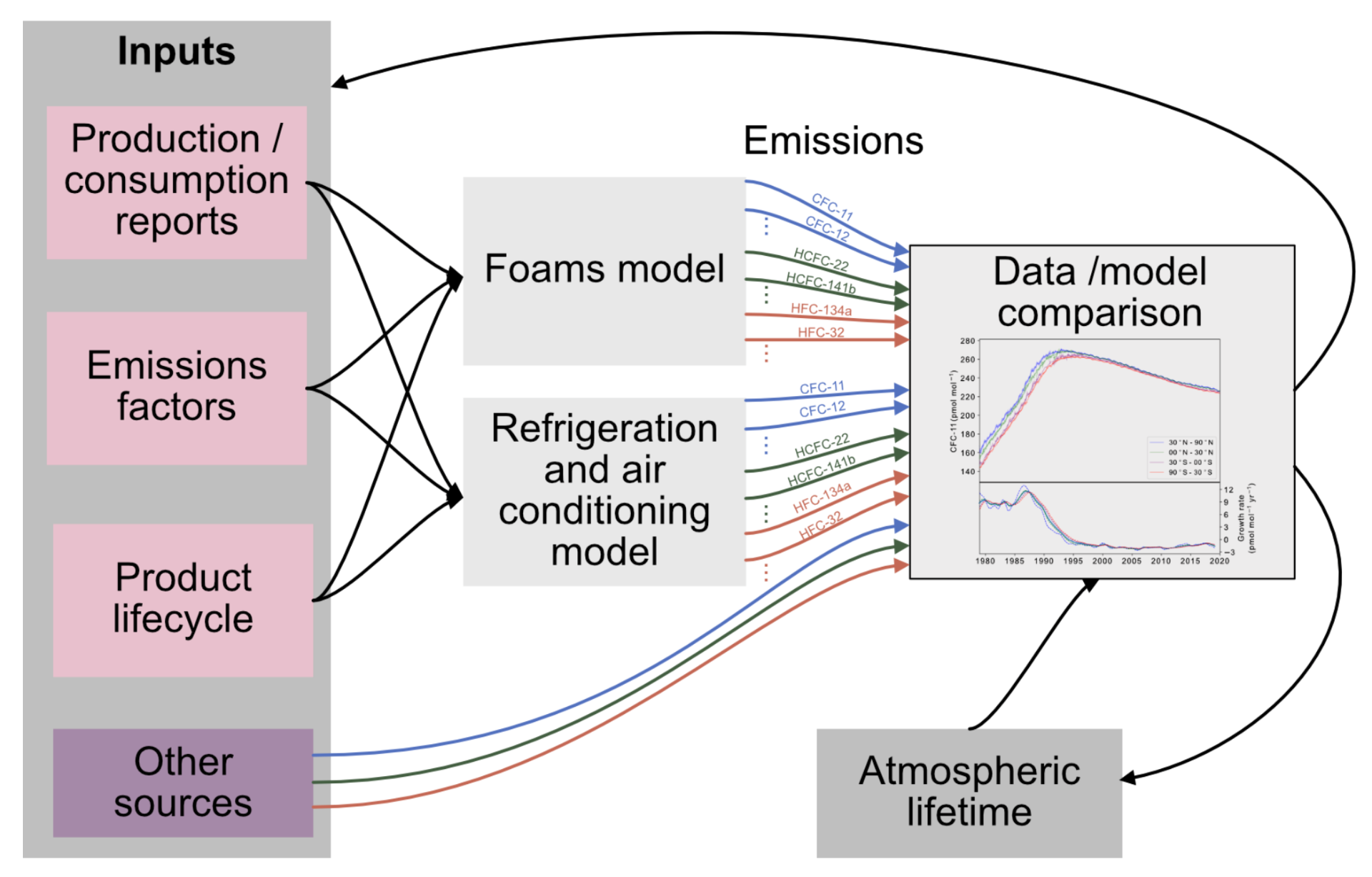
We will reconcile ODS production reports, magnitudes of banks and emissions at the global scale using a novel combined top-down and bottom-up framework. Recent work demonstrated this technique for CFC-11, -12 and -113, in which we applied a top-down method to infer parameters in a simplified bank model (Lickley et al., 2020). We will use atmospheric observations to examine and improve uncertain inputs to complex industry models of all the major ODSs and HFCs for the two major sectors relevant to substances regulated under the MP: foams, and refrigeration and air conditioning (RAC). These results will provide a new understanding of the relationship between production, banks, and emissions of ODSs and HFCs, allowing us to better assess the compliance of reported production with the objectives of the MP.

The overall approach is illustrated above: based on production and consumption reports, emissions factors, and industrial estimates of product lifecycles (e.g., lifespans, decommissioning processes, etc.), we will use foam and RAC models developed by industry experts to predict emissions of all the major regulated substances. These emissions will be input to the AGAGE 12-box model (a simplified 2D global model, e.g., Rigby et al., 2014), the concentrations from which can be compared to atmospheric observations. Using Gaussian process emulation methods that we have recently developed (Stell et al., 2020), combined with hierarchical Bayesian inference, we can explore the subset of model inputs that is consistent with the atmospheric data in a single framework, reconciling atmospheric and industrial constraints.

For the foam sector, Anthesis-Caleb (consultants) have developed a mature model of global emissions and banks, which has been used extensively in IPCC and TEAP reports (e.g., Ashford, 2004). For the RAC sector, we will build a global version of the Gluckman Consulting regional HFC Outlook model, a bottom-up stock model. These estimates will be inter-compared with recent TEAP models that are aiming to better understand ODS banks, ensuring that our work will feed into upcoming TEAP assessments.

To effectively constrain these models, a complete atmospheric record of the major ODSs and HFCs is required. We are now able to reconstruct and regularly update atmospheric abundances by combining measurements of firn air (provided by Empa and Scripps Institution of Oceanography, interpreted using the CSIRO firn model, see LoS from Empa, SIO and CSIRO), archived samples, and high frequency in situ measurements and flask samples made in the modern atmosphere by AGAGE, NOAA and other programmes.

Following the approach developed in Montzka et al. (2021), we will derive transport-related adjustments to emissions derived in the AGAGE 12-box model for the compounds CFC-11, -12, 113, HCFC-22, -141b, -142b, HFC-23, -134a, -125. This will be achieved by running the global 3D model, TOMCAT (e.g., Wilson et al., 2014), with several versions of each tracer based on different emissions (spatially varying, global mean and zero) derived from the 12-box model. Short timescale (~annual) differences between the TOMCAT-predicted mole fractions and those from the 12-box of focus on in the emissions, 9 model provide an insight into the effects of transport processes that are not accounted for by the 2D model. Adjustments to the derived global emissions can then be made to remove these biases.

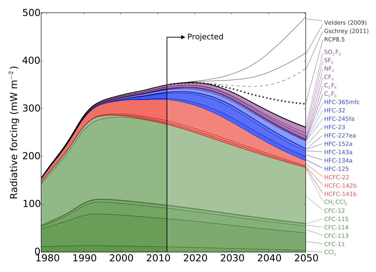
The major outcomes of this work will be improved estimates of bank sizes and release rates and, therefore, improved estimates of future emission trends (e.g., plot below, Rigby et al., 2014). Importantly, by integrating emission models into the data assimilation framework for the first time for most gases, we will have new understanding of whether emissions trends are plausible, given reported production.

The outputs of this activity will be updated and published annually. Currently, halocarbon emissions estimates are only routinely updated every 4-years as part of the Ozone Assessment cycle. To provide stakeholders and other researchers with more rapid updates, we will publish annual, global halocarbon budgets in an open-source living data platform such as Earth System Science Data (ESSD).

Predicted Radiative forcing from ozone depleting substances and greenhouse gases. Rigby et al., 2014

WP 2.2: Global 3D model emission estimates

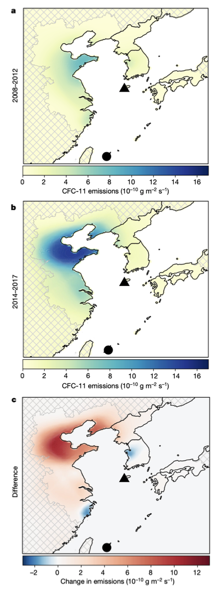
To derive emissions estimates around the world, the TOMCAT 4D-var data assimilation approach (Wilson et al., 2014) will be applied to AGAGE and NOAA data, and the new observations collected in WP 1. The key aim is to provide new insights on source regions that have not been quantified from recent studies, which have all been carried out at either global-total or regional scales. In particular, we will examine: a) whether the remaining ~50% of the recent global CFC-11 emission increase can be attributed to emissions from some region outside of eastern China, b) the origin of the discrepancy between global HFC-23 emissions and bottom-up estimates (Stanley et al., 2020), c) whether HFC emission reports to the UNFCCC from the last decade are consistent with atmospheric data (since previous global updates in, e.g., Lunt et al., 2015), d) whether regional emissions of carbon tetrachloride are consistent with bottom-up estimates and updated knowledge of atmospheric sinks (e.g. Chipperfield et al., 2016).

WP 2.3: Regional 3D model emission estimates

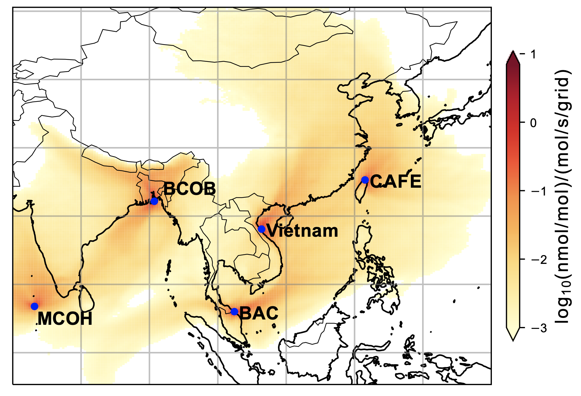
We will use UK Met Office Numerical Atmospheric-dispersion Modelling Environment (NAME, image of output below) with the hierarchical Bayesian emissions inference system developed by the University of Bristol (HBMCMC) and Inversion Technique for Emissions Modelling (InTEM) to provide new insights on the emissions of halocarbons from key regions. InHALE will derive regional emissions for South and East Asia using the new measurements in WP 1, focusing on compounds for which substantial gaps in the global budgets have been identified (e.g., CFC-11, HFCs including HFC-23; Montzka and Velders et al., 2018, Stanley et al., 2020).

Annual mean “footprints” (sensitivities of observations to emissions from the surrounding region) for InHALE flask sampling locations in East and South Asia calculated using the Met Office NAME model.

Eastern Asian emissions of CFC-11 inferred from atmospheric data (Rigby, et al., 2019) for the periods a) 2008 – 2012 and, b) 2014 – 2017. The difference (c), shows that emissions increased in eastern China, despite the 2010 global production ban.

We will add new capability to our regional inverse modelling approach by building time-resolved NAME “footprints” into our inversion frameworks. This will allow us to estimate emissions of HFOs for the first time in many parts of the world. The short atmospheric lifetime of HFOs precludes the use of “time integrated” footprints that have been used in previous studies (e.g., Rigby et al., 2019, see right).

The new data from WP 1 can be combined with existing measurements to provide new constraints on emissions from South and East Asia. The InHALE measurements from the Maldives and Bangladesh will allow us to develop the first multi-year estimate of emissions from parts of south Asia. We will use the NAME inverse modelling frameworks to determine the added value of the new measurements in Vietnam in quantifying emissions from southern China. These regional emissions estimates from the HBMCMC and InTEM systems will be compared to the TOMCAT 4D-var estimates from WP 2.2, to provide an assessment of transport model-related differences.

References

Ashford, 2004, Int. J. Refrig.

Chipperfield et al., 2016, Atmos. Chem. Phys., 16, 15741-15754;

Lickley et al., 2020, Nat. Commun., 11, 1380;

Lunt et al., 2015, PNAS, 112 (19), 5927-5931;

Montzka et al., 2021, Nat., 590, 428-432;

Montzka and Velders et al., 2018, Hydrofluorocarbons (HFCs), Chapter 2 in Scientific Assessment of Ozone Depletion: 2018;

Rigby et al., 2014, Geophys. Res. Lett., 41, 2623-2630;

Rigby et al., 2019, Nat., 569, 546-550;

Stanley et al., 2020, Nat. Commun., 11, 397;

Stell et al., 2021, Atmos. Chem. Phys., 21, 1717􏰒1736;

Wilson et al., 2014, Geosci. Mod. Dev. 7, 2485-2500;